The Optimal Control Theory in Control System
Optimal Control is a branch of control theory in control systems. The theory works by solving an optimization problem of a dynamical system in order to find the optimal solution for the system.
What is Model Predictive Control?
Model Predictive Control (MPC) is an optimal control method that uses optimization algorithms to minimize a cost function arising from a desired input and obtain the optimal control input over finite or infinite horizons. Recently, MPC has been widely adopted among control systems researchers for its speed, efficiency, and robustness in high-complexity systems.
Hamilton–Jacobi–Bellman Equation (HJBE)
HJBE is a nonlinear partial differential equation encoding necessary conditions for optimality by minimizing the loss function of the system.
We define the Hamiltonian:
Where:
- — number of prediction horizons (shooting nodes).
- — state at node .
- — input at node .
- — (typically diagonal) weighting matrices.
- — state transition dynamics.
- — equality/inequality constraint functions.
- — costate vector.
- — Lagrange multipliers for constraints.
Nonlinear MPC has multiple solving methods; here we focus on the Continuation/GMRES method proposed by Prof. Toshiyuki Ohtsuka.
Suppose we want the solution vector at sampling time :
We define the discretized Euler–Lagrange equations (ELE). To solve the resulting nonlinear system iteratively, we use Newton’s method on where stacks the stationarity conditions over the horizon:
Directly solving this is expensive; Continuation reduces complexity and then we apply GMRES.
Continuation
Let . Define the continuation dynamics for :
Define finite-difference approximations:
Generalized Minimal Residual Method (GMRES)
GMRES is an iterative method for solving large, sparse linear systems . The Arnoldi process builds an orthonormal Krylov basis and an upper-Hessenberg matrix , then one solves a least-squares problem to minimize the residual.
Sketch:
- Choose , compute set .
- For : perform Arnoldi to get and .
- Solve .
- Update . For a differential-drive model with state and dynamics , we can define:
- constraints (e.g., box constraints on )
- terminal penalty
Then,
Implementing in Python
It is safe to say that you will need to start from basic first. Like creating class for model representation, but for now I will just go with CGMRES implementing only, since I have done many demonstration of how to create class for model.
Let's create class for Hamiltion Jacobian Bellman Equation which we already derived from above equation.
class HJBEquation:

    def __init__(self, q1, q2, q3, r1, r2, u_max, u_min):

        self.q1 = q1
        self.q2 = q2
        self.q3 = q3

        self.r1 = r1
        self.r2 = r2

        self.u1_min = u_min[0]
        self.u2_min = u_min[0]

        self.u1_max = u_max[0]
        self.u2_max = u_max[1]

    def dhdx(self, x, y, yaw, x_r, y_r, yaw_r, u1, lam1, lam2):

        dhdx1 = (x-x_r)*self.q1
        dhdx2 = (y-y_r)*self.q2
        dhdx3 = (yaw-yaw_r)*self.q3-u1*lam1*np.sin(yaw)+u1*lam2*np.cos(yaw)

        return dhdx1, dhdx2, dhdx3

    def dhdu(self, yaw, u1, u2, u1_r, u2_r, lam1, lam2, lam3, mu1, mu2):

        dhdu1 = self.r1*(u1-u1_r)+lam1*np.cos(yaw)+lam2*np.sin(yaw)+2*mu1*u1*(u1+(self.u1_max+self.u1_min)/2)
        dhdu2 = self.r2*(u2-u2_r)+lam3+2*mu2*(u2+(self.u2_max+self.u2_min)/2)

        return dhdu1, dhdu2

    def dphidx(self, x, y, yaw, x_r, y_r, yaw_r):
        dphidx1 = self.q1*(x-x_r)
        dphidx2 = self.q2*(y-y_r)
        dphidx3 = self.q3*(yaw-yaw_r)

        return dphidx1, dphidx2, dphidx3
Here, I suggest that you should understand the mathematics equations above that I try to explain. It is easy to do it in Python programming language if you already understand its expression. Now I created another class for NMPC with CGMRES.
class NMPCCGMRES:

    def __init__(self):

        ## NMPC params
        self.x_dim = 3
        self.u_dim = 2
        self.c_dim = 2
        self.pred_horizons = 10

        ### Continuations Params
        self.ht = 1e-5
        self.zeta = 1/self.ht
        self.alpha = 0.5
        self.tf = 1.0

        ### Matrix

        self.q1 = 1
        self.q2 = 6
        self.q3 = 1
        self.r1 = 1
        self.r2 = 0.1

        ### Constraint
        self.u_min = [ 0,  0]
        self.u_max = [ 2,  1.57]
        self.u_dummy = [0.01, 0.01]

        ### Initialize matrix solution
        self.dU = np.zeros((self.u_dim, self.pred_horizons))

        ### Reference point
        self.X_r = [3, 2, 0.0]
        self.U_r = [0, 0]
These are just for tuning parameters and initialize parameters, let's focus on CGMRES method. As the expression above at equation (1). Let's denote that
X = np.zeros((x_dim, pred_horizons+1))      ## State for N-prediction+1
U = np.zeros((u_dim, pred_horizons))        ## Input Control for N-prediction
Lambda = np.zeros((x_dim, pred_horizons+1)) ## Costate vector for N-prediction+1
dt = 0.01                                   ## Sampling Time
Then, we can perform equation (1) as
def calc_state(self, X, U, dt):

        for i in range(self.pred_horizons):
            x_dot, y_dot, yaw_dot = self.robot_model.forward_kinematic(X[2, i], U[0, i], U[1, i])

            X[0, i+1] = X[0, i] + x_dot * dt
            X[1, i+1] = X[1, i] + y_dot * dt
            X[2, i+1] = X[2, i] + yaw_dot * dt

        return X
Next we calculating costate, we are going in backward direction
def calc_costate(self, X, U, Lambda, dt):

        x_N, y_N, yaw_N = self.hjb_equation.dphidx(X[0, -1], X[1, -1], X[2, -1],
                                                   self.X_r[0], self.X_r[1], self.X_r[2])
        Lambda[0, -1] = x_N
        Lambda[1, -1] = y_N
        Lambda[2, -1] = yaw_N

        for i in reversed(range(1, self.pred_horizons)):

            dhdx1, dhdx2, dhdx3 = self.hjb_equation.dhdx(
                X[0, i], X[1, i], X[2, i],
                self.X_r[0], self.X_r[1], self.X_r[2],
                U[0, i], Lambda[0, i+1], Lambda[1, i+1]
            )

            Lambda[0, i] = Lambda[0, i+1] + dhdx1 * dt
            Lambda[1, i] = Lambda[1, i+1] + dhdx2 * dt
            Lambda[2, i] = Lambda[2, i+1] + dhdx3 * dt


        return Lambda
And finally, calculating Newton F Function
def calc_f(self, X, U, Lambda, Mu, dt):

        X_new = self.calc_state(X, U, dt)

        Lambda_new = self.calc_costate(X_new, U, Lambda, dt)

        F = np.zeros((self.u_dim, self.pred_horizons))

        for i in range(self.pred_horizons):
            dhdu1, dhdu2 = self.hjb_equation.dhdu(X_new[2, i], U[0, i], U[1, i],
                                                  self.U_r[0], self.U_r[1],
                                                  Lambda_new[0, i+1], Lambda_new[1, i+1], Lambda_new[2, i+1],
                                                  Mu[0, i], Mu[1, i])
            F[0, i] = dhdu1
            F[1, i] = dhdu2

        F = F.T.ravel().reshape(-1, 1)

        return F
Now let's introduce Continuation method for Function F, you can look at the Continuation part.
# Time step horizons
dt = self.tf * (1-np.exp(-self.alpha*time)) / self.pred_horizons
# F(x,u,t+h)
F = self.calc_f(X, U, Lambda, Mu, dt)
# F(x+hdx,u,t+h)
x_dot, y_dot, yaw_dot = self.robot_model.forward_kinematic(X[2, 0], U[0, 0], U[1, 0])
X[:, 0] = X[:, 0] + np.array([x_dot, y_dot, yaw_dot]) * self.ht
Fxt = self.calc_f(X, U, Lambda, Mu, dt)
# F(x+hdx,u+hdx,t+h)
Fuxt = self.calc_f(X, U + self.dU*self.ht, Lambda, Mu , dt)

# Define right-left handside equation
left = (Fuxt - Fxt) / self.ht
right = -self.zeta * F - (Fxt - F)/self.ht
Here is the crucial part, we need to implement GMRES solver for our *F function to obtain solution vector.
# Define right-left handside equation
left = (Fuxt - Fxt) / self.ht
right = -self.zeta * F - (Fxt - F)/self.ht

# Define iterations
m = (self.u_dim ) * self.pred_horizons
# Define r0
r0 = right - left
# print(r0)

# GMRES
Vm = np.zeros((m, m+1))
Vm[:, 0:1] = r0 / np.linalg.norm(r0)
# print("Vm", Vm[:, 0])
Hm = np.zeros((m+1, m))
# print(Vm[:, 0])

for i in range(m):
    Fuxt = self.calc_f(
        X, U + Vm[:, i:i+1].reshape(self.u_dim, self.pred_horizons, order='F') * self.ht,
        Lambda, Mu,
        dt
    )

    Av = (Fuxt - Fxt) / self.ht

    for k in range(i+1):
        Hm[k, i] = np.dot(Av.T, Vm[:, k:k+1])

    temp_vec = np.zeros((m, 1))

    for k in range(i+1):
        temp_vec = temp_vec + np.dot(Hm[k, i], Vm[:, k:k+1])

    v_hat = Av - temp_vec

    Hm[i+1, i] = np.linalg.norm(v_hat)

    Vm[:,i+1:i+2] = v_hat/Hm[i+1, i]

e = np.zeros((m+1, 1))
e[0, 0] = 1.0
gm = np.linalg.norm(r0) * e
# print(gm)

UTMat, gm = self.ToUTMat(Hm, gm, m)

min_y = np.zeros((m, 1))

for i in range(m):
    min_y[i][0] = (gm[i, 0] - np.dot(UTMat[i:i+1 ,:] ,min_y))/UTMat[i, i]

dU_new = self.dU + np.dot(Vm[:, 0:m], min_y).reshape(self.u_dim, self.pred_horizons, order='F')

self.dU = dU_new

U = U + self.dU * self.ht
You can look in my code inside function solve_nmpc.
Experiment in Python
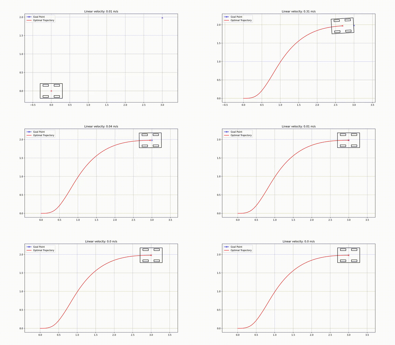
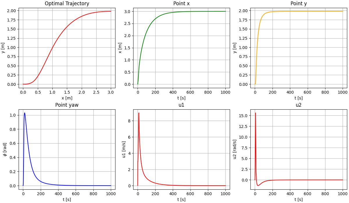
GMRES was consider one of the fastest solver for sparse linear algebra problem, so I will include the link for the GMRES algorithms. In my experiment, I use differential drive robot.
Consider as our state representation and of course setting , also
Animation:
Simulation Plots:
Conclusion
Nonlinear MPC with CGMRES offers very fast numerical computation thanks to GMRES with Givens rotations. Compared to other NMPC solvers, CGMRES can be sensitive to parameter tuning and may exhibit unstable numerical behavior if not tuned carefully. Multiple-shooting variants are often more numerically robust than single-shooting.
References
- A real-time algorithm for nonlinear receding horizon control using multiple shooting and continuation/Krylov method
- Nonlinear Model Predictive Control with CGMRES of Steering Car
- C/GMRES シミュレーションを3つの言語で作ったので比較してみた
- Krylov 部分空間と GMRES 法について (Qiita)
- Nonlinear Model Predictive Control of Position and Attitude in a Hexacopter with Three Failed Rotors