What is PID Controller?
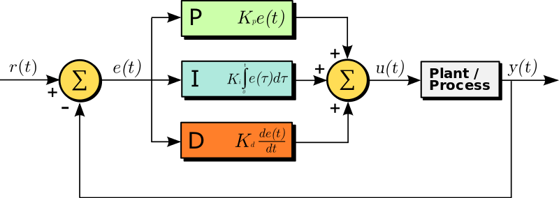
The Proportional–Integral–Derivative (PID) controller is a classic feedback controller that’s been widely used since the 1940s in control engineering and industrial applications. A PID controller minimizes the error between the system’s feedback and the desired setpoint by tuning the gains .
How it works?
Imagine controlling a DC motor to reach 300 RPM. Because of the motor’s natural dynamics, it won’t instantly hit the target. A PID controller shapes the time response (rise time, overshoot, settling) using three terms that act on the error signal.
Formulation
- — proportional gain
- — integral gain
- — derivative gain
- — tracking error
Response Time
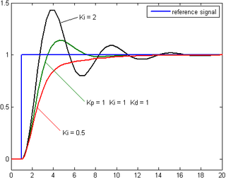
Observations (from the figure):
- With : likely overshoot before steady state — undesirable for some applications (e.g., DC motor).
- With : slower response, little/no overshoot.
- With : slight overshoot and faster settling.
How can we write PID code in Python?
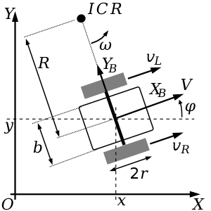
We’ll use a differential-drive robot as a case study (common in robotics & automation).
Python classes
class DifferentialDrive:
    def __init__(self):
        self.r = 0.05
        self.L = 0.25

    def forward_kinematic(self, v, omega, yaw):
        vx = v * np.cos(yaw)
        vy = v * np.sin(yaw)
        vyaw = omega
        return vx, vy, vyaw

    def discrete_state(self, x, y, yaw, v, omega, dt):
        dx, dy, dyaw = self.forward_kinematic(v, omega, yaw)
        x_next = x + dx * dt
        y_next = y + dy * dt
        yaw_next = yaw + dyaw * dt
return x_next, y_next, yaw_nextclass PIDController:
def __init__(self, kp, ki, kd, dt):
self.kp = kp
self.ki = ki
self.kd = kd
self.dt = dt
self.integral = 0
def calculate_pid(self, errors):
proportional = self.kp * errors[-1]
integral = self.integral + self.ki * errors[-1] * self.dt
self.integral = integral
derivative = self.kd * (errors[-1] - errors[-2]) / self.dt
output = proportional + integral + derivative
return outputExperiment
PID for point control
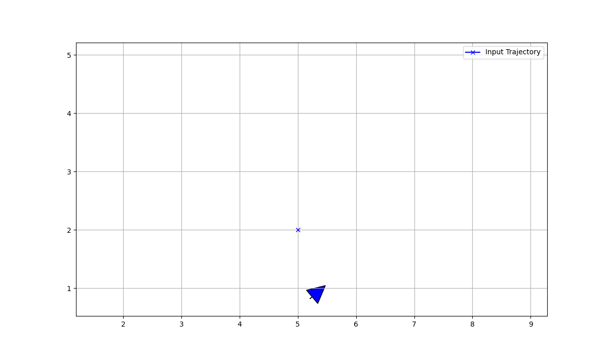
Goal: drive the robot to a reference point . Compute errors recursively:
error_x.append(ref_path[0] - current_x)
error_y.append(ref_path[1] - current_y)
error_yaw.append(ref_path[2] - current_yaw)

output_vx   = pid_controller_x.calculate_pid(error_x)
output_vy   = pid_controller_y.calculate_pid(error_y)
output_omega= pid_controller_yaw.calculate_pid(error_yaw)

x_next, y_next, yaw_next = diff_drive.discrete_state(
    current_x, current_y, current_yaw, v_pid, omega_pid, sampling_time
)
Visualization snippet:
plt.clf()
plt.gcf().canvas.mpl_connect(
    'key_release_event',
    lambda event: [exit(0) if event.key == 'escape' else None]
)
plot_arrow(current_x, current_y, current_yaw)
plt.plot(5, 5)
plt.plot(ref_path[0], ref_path[1], marker="x", color="blue", label="Input Trajectory")
plt.axis("equal")
plt.grid(True)
plt.legend()
plt.pause(0.0001)
Path Tracking
Same idea as point control, but feed a sequence of waypoints (a spline path). Full code here: PathTracking/PID.
Result
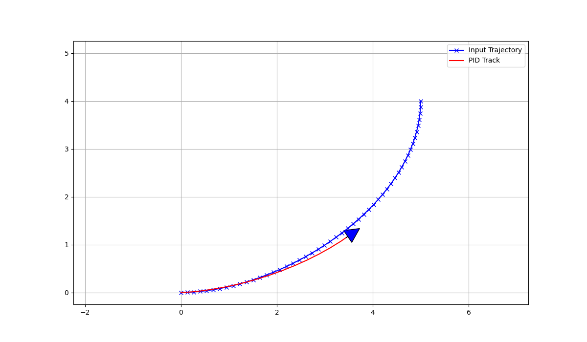
In Conclusion
PID remains a great first-choice controller for many applications because it is simple yet capable of handling a wide range of control tasks when properly tuned.